The t-test is a foundational statistical hypothesis test used to determine if there is a significant difference between the means of two groups, which may be related in certain features.
It is applied when the test statistic follows a normal distribution and the value of a scaling term in the test statistic follows a Student’s t-distribution under the null hypothesis.
The t-test is most commonly applied when the test statistic would follow a normal distribution if the value of a scaling term in the test statistic were known. When the scaling term is unknown and is replaced by an estimate based on the data, the test statistics (under certain conditions) follow a Student’s t distribution.
When to use T test
Small Samples: The T-test extends the principles learned from the Z-test to situations where the sample size is small (usually n < 30) and the population variance is unknown. It introduces the concept of using sample data to estimate population parameters, adding a layer of complexity.
Student’s T-Distribution: The T-test introduces a new distribution, the T-distribution, which is more spread out than the Z-distribution, especially for small sample sizes. The shape of the T-distribution changes with the degrees of freedom, a concept not encountered with the Z-distribution.
8.1.1 Concept of Degrees of Freedom in T-Tests
Degrees of freedom (df) in statistics generally refer to the number of values in a calculation that are free to vary without violating any constraints.
In the context of a t-test, degrees of freedom are crucial for determining the specific distribution of the t-statistic under the null hypothesis.
A t-test is used to determine if there is a significant difference between the means of two groups under the assumption that the data follows a normal distribution but when the population standard deviation is not known.
The t-test uses the sample standard deviation as an estimate of the population standard deviation. This estimation introduces more variability and uncertainty, which is why the t-distribution, rather than the normal distribution, is used.
The t-distribution is wider and has thicker tails than the normal distribution, which accounts for this additional uncertainty.
8.1.2 Why Z-Tests don’t have Degrees of Freedom 🤔 ?
The Z-test, unlike the t-test, does not involve degrees of freedom because it uses the population standard deviation (\(\sigma\)), which is assumed to be known.
Because the Z-test uses the actual population standard deviation and not an estimate from the sample, there is no extra uncertainty introduced by estimation that needs to be accounted for using degrees of freedom.
Consequently, the distribution of the Z-test statistic under the null hypothesis is the standard normal distribution (Z-distribution), which is not dependent on the sample size once the population standard deviation is known.
8.1.3 Types of T-Tests
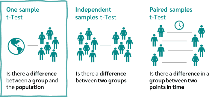
There are three main types of t-tests, each suited for different testing scenarios:
One-sample t-test: This test compares the mean of a single group against a known standard or mean. For instance, it could be used to determine if the average process time for completing a task is different from the standard time.
Independent Samples t-test: This test compares the means of two independent groups in order to determine whether there is statistical evidence that the associated population means are significantly different. It is used when the variances of two normal distributions are unknown and the samples are independent. A common example is comparing the test scores of two different groups of students.
Paired Samples t-test: This test is used to compare the means of the same group or related samples at two different points in time or under two different conditions. It’s often used in before-and-after studies, such as measuring the effect of a training program on the performance of athletes by measuring them before and after the program.
The t-test has widespread applications across various fields such as:
Education: To compare test scores, teaching methods, or learning outcomes.
Medicine: For assessing the effectiveness of treatments or drugs.
Manufacturing and quality control: To determine if the process changes have led to improvements.
Social sciences: To compare differences in social, psychological, or behavioral effects across groups.
Assumptions
For the t-test to be valid, certain assumptions must be met:
Independence of Observations: Each observation must be independent of all other observations.
Normality: The data should be approximately normally distributed, especially as the sample size increases (Central Limit Theorem).
Equality of Variances (for independent samples t-test): The variances of the two groups being compared should be equal. When this assumption is violated, a variation of the t-test called Welch’s t-test can be used.
Interpretation
The output of a t-test is a p-value, which indicates the probability of observing the test results under the null hypothesis. If the p-value is below a predetermined threshold (commonly 0.05), the null hypothesis is rejected, indicating that there is a statistically significant difference between the groups being compared.
The t-test is a robust tool with wide applicability but must be used judiciously, respecting its assumptions for valid results. Advances in statistical methodologies have introduced more complex models for data analysis, yet the t-test remains a fundamental and widely used method for comparing means.
Degrees of freedom in different types of t-tests:
One-Sample t-test: df = n - 1, where \(n\) is the number of observations in the sample. Subtracting one accounts for the estimation of the sample mean from the sample data itself.
Independent Two-Sample t-test: df = \(n_1\) + \(n_2\) - 2, where \(n_1\) and \(n_2\) are the sample sizes of the two groups. Here, two degrees are lost because each group’s mean is estimated from its sample.
Paired t-test: df = n - 1. In paired samples, each pair’s difference is considered as a single piece of data. If there are \(n\) pairs, the degrees of freedom are n - 1, reflecting the \(n\) paired differences.
8.1.4 One-Sample T-Test
The one-sample t-test is a statistical procedure used to determine whether the mean of a single sample differs significantly from a known or hypothesized population mean. This test is particularly useful when the population standard deviation is unknown and the sample size is small, which is a common scenario in many practical research applications.
Assumptions
Before conducting a one-sample t-test, certain assumptions must be verified to ensure the validity of the test results:
Normality: The data should be approximately normally distributed. This assumption is especially important with smaller sample sizes. For larger samples, the Central Limit Theorem helps as it suggests that the means of the samples will be approximately normally distributed regardless of the shape of the population distribution.
Independence: The sampled observations must be independent of each other. This means that the selection of one observation does not influence or alter the selection of other observations.
Scale of Measurement: The data should be measured at least at the interval level, which means that the numerical distances between measurements are defined.
Formula
The t-statistic is calculated using the formula:
\[t = \frac{\bar{x} - \mu_0}{s / \sqrt{n}}\]
Where:
\(\bar{x}\) is the sample mean.
\(\mu_0\) is the hypothesized population mean.
\(s\) is the sample standard deviation.
\(n\) is the sample size.
Calculating Degrees of Freedom
The degrees of freedom for the one-sample t-test are calculated as \(n - 1\). This value is crucial for determining the critical values from the t-distribution, which are needed to assess the significance of the test statistic.
Interpretation
To decide whether to reject the null hypothesis, compare the calculated t-value to the critical t-value from the t-distribution at the desired significance level (\(\alpha\), often 0.05 for a 5% significance level). The decision rules are:
If the absolute value of the calculated t-value is greater than the critical t-value, reject the null hypothesis.
If the absolute value of the calculated t-value is less than or equal to the critical t-value, do not reject the null hypothesis.
One-Sample T-Test Example problem
A bakery claims that its chocolate chip cookies weigh at least 60 grams on average. A quality control manager is skeptical of this claim and decides to test it. She randomly selects 15 cookies and finds the following weights in grams:
She decides to use a one-sample t-test to see if there’s evidence that the average weight is different from the bakery’s claim. She chooses a significance level of 0.05.
Hypotheses
Null Hypothesis (\(H_0\)): \(\mu = 60\) grams. The average weight of the cookies is 60 grams.
Alternative Hypothesis (\(H_1\)): \(\mu \neq 60\) grams. The average weight of the cookies is not 60 grams.
First, let’s calculate the sample mean (\(\bar{x}\)), sample standard deviation (\(s\)), and the t-statistic.
Calculate the Sample Mean (\(\bar{x}\)):
The sample size \(n\) is 15.
Sample mean = \[
\bar{x} = \frac{\sum \text{sample values}}{n}
\]
Based on the t-statistic, look up or compute the p-value for \(|t| = 2.32\) with \(df = 14\). This value is approximately \(p = 0.036\).
Interpretation
T-Statistic: The negative value of the t-statistic (-2.32) indicates that the sample mean is less than the null hypothesis mean of 60 grams.
P-Value: The p-value of 0.036 is less than the chosen significance level of 0.05. This suggests that there is statistically significant evidence to reject the null hypothesis.
Therefore, based on the sample of 15 cookies, there is sufficient statistical evidence to conclude that the average weight of the bakery’s chocolate chip cookies is different from the claimed 60 grams.
Given the direction indicated by the t-statistic, it suggests that the cookies may, on average, weigh less than the claimed 60 grams.
# Calculate sample standard deviation (R uses n-1 by default)sample_sd<-sd(weights)sample_sd
[1] 3.453087
Code
# Define population mean for comparisonpopulation_mean<-60population_mean
[1] 60
Code
# Calculate the t-statistict_statistic<-(sample_mean-population_mean)/(sample_sd/sqrt(sample_size))t_statistic
[1] -2.317974
Code
# Degrees of freedomdegrees_of_freedom<-sample_size-1degrees_of_freedom
[1] 14
Code
# Calculate the p-value for a two-tailed testp_value<-2*pt(-abs(t_statistic), df =degrees_of_freedom)p_value
[1] 0.03609761
Code
# Decision based on p-valueif(p_value<alpha){cat("Reject null hypothesis\n")}else{cat("Do not reject null hypothesis\n")}
Reject null hypothesis
8.1.5 Independent samples t-test / Two Sample t-test
The independent samples t-test, also known as the two-sample t-test or Student’s t-test, is a statistical procedure used to determine if there is a significant difference between the means of two independent groups. This test is commonly used in situations where you want to compare the means from two different groups, such as two different treatments or conditions, to see if they differ from each other in a statistically significant way.
Assumptions
You would use an independent samples t-test under the following conditions:
Independence of Samples: The two groups being compared must be independent, meaning the samples drawn from one group do not influence the samples from the other group.
Normally Distributed Data: The data in the two groups should be roughly normally distributed.
Equality of Variances: The variances of the two groups are assumed to be equal. If this assumption is significantly violated, a variation of the t-test, like Welch’s t-test, may be used instead.
Hypotheses
The hypotheses for an independent samples t-test are usually framed as follows:
Null Hypothesis (H₀): The means of the two groups are equal (\(\mu_1 = \mu_2\)).
Alternative Hypothesis (H₁): The means of the two groups are not equal (\(\mu_1 \neq \mu_2\)), which can be two-tailed, or one-tailed if the direction of the difference is specified.
Formula
The t-statistic is calculated using the following formula: \[
t = \frac{\bar{X}_1 - \bar{X}_2}{s_p \cdot \sqrt{\frac{1}{n_1} + \frac{1}{n_2}}}
\] Where:
\(\bar{X}_1\) and \(\bar{X}_2\) are the sample means of groups 1 and 2, respectively.
\(n_1\) and \(n_2\) are the sample sizes of groups 1 and 2, respectively.
\(s_p\) is the pooled standard deviation of the two samples, calculated as: \[
s_p = \sqrt{\frac{(n_1 - 1) \cdot s_1^2 + (n_2 - 1) \cdot s_2^2}{n_1 + n_2 - 2}}
\]
\(s_1^2\) and \(s_2^2\) are the variances of the two samples.
Calculating Degrees of Freedom
The degrees of freedom used in this table are \(n_1 + n_2 - 2\).
Interpretation
To decide whether to reject the null hypothesis, compare the calculated t-value to the critical t-value from the t-distribution at the desired significance level (\(\alpha\), often 0.05 for a 5% significance level). The decision rules are:
If the absolute value of the calculated t-value is greater than the critical t-value, reject the null hypothesis.
If the absolute value of the calculated t-value is less than or equal to the critical t-value, do not reject the null hypothesis.
This test allows researchers to understand whether different conditions have a statistically significant impact on the means of the groups being compared, providing crucial insights in fields such as medicine, psychology, and economics.
Two Samples T-Test Example problem
Suppose we want to determine if there is a significant difference in the average test scores between two classes. Class A has 5 students, and Class B has 5 students. Here are their test scores:
Class A: 85, 88, 90, 95, 78
Class B: 80, 83, 79, 92, 87
Hypotheses:
Null Hypothesis (H₀): \(\mu_1 = \mu_2\) (The means of both classes are equal)
Alternative Hypothesis (H₁): \(\mu_1 \neq \mu_2\) (The means of both classes are not equal)
We will use a significance level (\(\alpha\)) of 0.05.
To illustrate the mathematics behind the calculations performed for the independent samples t-test, let’s break down each step using the provided scores for Class A and Class B:
Calculate the means (\(\bar{X}_1\) and \(\bar{X}_2\)):
For Class A: \[ \bar{X}_1 = \frac{85 + 88 + 90 + 95 + 78}{5} = 87.2 \]
For Class B: \[ \bar{X}_2 = \frac{80 + 83 + 79 + 92 + 87}{5} = 84.2 \]
Calculate the sample variances (\(s_1^2\) and \(s_2^2\)):
\[ t = \frac{87.2 - 84.2}{\sqrt{34.2} \cdot \sqrt{\frac{1}{5} + \frac{1}{5}}} \]\[ t = \frac{3}{\sqrt{34.2} \cdot \sqrt{\frac{2}{5}}} \]\[ t = \frac{3}{\sqrt{34.2} \cdot \sqrt{0.4}} \]\[ t = \frac{3}{5.85 \cdot 0.6325} = 0.8111 \]
Degrees of freedom:
\[ \text{df} = 5 + 5 - 2 = 8 \]
The critical t-value and p-value:
The t-value needs to be compared against the critical value from a t-distribution table for df = 8 and a two-tailed test with \(\alpha = 0.05\).
If t > 2.306, the null hypothesis is rejected.
In this case, t = 0.8111, so the null hypothesis is not rejected.
# Test scores for two independent classesclass_a_scores<-c(85, 88, 90, 95, 78)class_b_scores<-c(80, 83, 79, 92, 87)alpha=0.05# Perform independent samples t-test# We assume equal variances for this example with var.equal = TRUEt_test_result<-t.test(class_a_scores, class_b_scores, var.equal =TRUE)# Print the resultst_test_result
    Two Sample t-test

data:  class_a_scores and class_b_scores
t = 0.81111, df = 8, p-value = 0.4408
alternative hypothesis: true difference in means is not equal to 0
95 percent confidence interval:
 -5.529099 11.529099
sample estimates:
mean of x mean of y
     87.2      84.2
Code
p_value=t_test_result$p.valueif(p_value<alpha){cat("Reject null hypothesis\n")}else{cat("Do not reject null hypothesis\n")}
Do not reject null hypothesis
Example Research Articles on Independent samples t-test:
The paired sample t-test, also known as the dependent sample t-test or repeated measures t-test, is a statistical method used to compare two related means. This test is applicable when the data consists of matched pairs of similar units or the same unit is tested at two different times.
Key Features and Applications
The paired sample t-test is commonly used in situations such as:
Comparing the before and after effects of a treatment on the same subjects.
Measuring performance on two different occasions.
Comparing two different treatments on the same subjects in a crossover study.
Assumptions
To properly conduct a paired sample t-test, the data must meet the following assumptions:
Paired Data: The observations are collected in pairs, such as pre-test and post-test measurements or measurements of the same subjects under two different conditions.
Normality: The differences between the paired observations should be approximately normally distributed. This assumption can be tested using plots or normality tests like the Shapiro-Wilk test.
Scale of Measurement: The variable being tested should be continuous and measured at least at the interval level.
Hypotheses
The hypotheses for a paired sample t-test are as follows:
Null Hypothesis (H₀): The mean difference between the paired observations is zero (\(\mu_d = 0\)).
Alternative Hypothesis (H₁): The mean difference between the paired observations is not zero (\(\mu_d \neq 0\)). This can be tailored to a one-tailed test if a specific direction is hypothesized (\(\mu_d > 0\) or \(\mu_d < 0\)).
Formulae
Mean Difference (\(\bar{d}\)):
The mean difference is calculated by taking the average of the differences between all paired observations. \[ \bar{d} = \frac{1}{n} \sum_{i=1}^n (x_{i1} - x_{i2}) \] Where \(x_{i1}\) and \(x_{i2}\) are the measurements from the first and second condition for the ith pair, and \(n\) is the number of pairs.
Standard Deviation of the Differences (\(s_d\)):
This measures the variability of the differences between the paired observations. \[ s_d = \sqrt{\frac{\sum_{i=1}^n (d_i - \bar{d})^2}{n-1}} \] Here, \(d_i = x_{i1} - x_{i2}\) represents the difference for each pair.
t-Statistic:
The t-statistic is calculated to determine if the differences are statistically significant. \[ t = \frac{\bar{d}}{s_d / \sqrt{n}} \] This formula represents the ratio of the mean difference to the standard error of the difference.
calculation of Degrees of Freedom
The degrees of freedom for the paired sample t-test are \(n - 1\), where \(n\) is the number of pairs.
Interpretation
To decide whether to reject the null hypothesis, compare the calculated t-value with the critical t-value from the t-distribution at the chosen significance level (\(\alpha\)), typically set at 0.05 for a 5% significance level. If the absolute value of the t-statistic is greater than the critical value, the null hypothesis is rejected, suggesting a significant difference between the paired groups.
This test is particularly valuable for detecting changes in conditions or treatments when the same subjects are observed under both scenarios, as it effectively accounts for variability between subjects.
Paired samples t-test Example problem
Let’s say a nutritionist wants to test the effectiveness of a new diet program. To do this, they measure the weight of 5 participants before starting the program and again after 6 weeks on the program. The goal is to see if there is a significant change in weight due to the diet.
Participant Weights (kg) Before the Diet: 70, 72, 75, 80, 78
Participant Weights (kg) After the Diet: 68, 70, 74, 77, 76
Hypotheses:
Null Hypothesis (H₀): There is no significant difference in the mean weight before and after the diet. (\(\mu_d = 0\))
Alternative Hypothesis (H₁): There is a significant difference in the mean weight before and after the diet. (\(\mu_d \neq 0\))
Significance Level:
We will use a significance level (\(\alpha\)) of 0.05.
Let’s break down the detailed mathematics behind each step of the paired samples t-test for the diet program effectiveness example, using the provided weights before and after the diet.
Use the formula for the t-statistic with \(n = 5\) (number of participants): \[
t = \frac{\bar{d}}{s_d / \sqrt{n}} = \frac{2}{0.707 / \sqrt{5}} = \frac{2}{0.707 / 2.236} = \frac{2}{0.316} = 6.324
\]
Degrees of freedom (\(df\)):
\[
df = n - 1 = 5 - 1 = 4
\]
Compare the calculated t-statistic to the critical t-value:
The critical t-value for \(df = 4\) and a two-tailed test with \(\alpha = 0.05\) is approximately 2.776 (from t-distribution tables).
Interpretation
Since the calculated t-statistic (6.324) is significantly greater than the critical t-value (2.776), we reject the null hypothesis. This indicates a statistically significant decrease in weight due to the diet, confirming the effectiveness of the nutritionist’s program. The precise calculation steps and their results provide strong mathematical evidence for this conclusion.
# Participant weights before and after the dietweights_before<-c(70, 72, 75, 80, 78)weights_after<-c(68, 70, 74, 77, 76)alpha=0.05# Perform paired samples t-testt_test_result<-t.test(weights_before, weights_after, paired =TRUE)# Print the resultst_test_result
    Paired t-test

data:  weights_before and weights_after
t = 6.3246, df = 4, p-value = 0.003198
alternative hypothesis: true mean difference is not equal to 0
95 percent confidence interval:
 1.122011 2.877989
sample estimates:
mean difference
              2
ANOVA, which stands for Analysis of Variance, is a statistical technique used to determine if there are any statistically significant differences between the means of three or more independent (unrelated) groups. It tests the hypothesis that the means of several groups are equal, and it does this by comparing the variance (spread) of scores among the groups to the variance within each group. The primary goal of ANOVA is to uncover whether there is a difference among group means, rather than determining which specific groups are different from each other.
8.2.1 Types of ANOVA
One-Way ANOVA: Also known as single-factor ANOVA, it assesses the impact of a single factor (independent variable) on a continuous outcome variable. It compares the means across two or more groups. For example, testing the effect of different diets on weight loss.
Two-Way ANOVA: This extends the one-way by not only looking at the impact of one, but two factors simultaneously on a continuous outcome. It can also evaluate the interaction effect between the two factors. For example, studying the effect of diet and exercise on weight loss.
Repeated Measures ANOVA: Used when the same subjects are used for each treatment (e.g., measuring student performance at different times of the year).
Multivariate Analysis of Variance (MANOVA): MANOVA is an extension of ANOVA when there are two or more dependent variables.
8.2.2 Assumptions of ANOVA
ANOVA relies on several assumptions about the data:
Independence of Cases: The groups compared must be composed of different individuals, with no individual being in more than one group.
Normality: The distribution of the residuals (differences between observed and predicted values) should follow a normal distribution.
Homogeneity of Variances: The variance among the groups should be approximately equal. This can be tested using Levene’s Test or Bartlett’s Test.
ANOVA Formula
The basic formula for ANOVA is centered around the calculation of two types of variances: within-group variance and between-group variance. The F-statistic is calculated by dividing the variance between the groups by the variance within the groups:
\[F = \frac{\text{Variance between groups}}{\text{Variance within groups}}\]
Steps to Conduct ANOVA
State the Hypothesis:
Null hypothesis (H0): The means of the different groups are equal.
Alternative hypothesis (Ha): At least one group mean is different from the others.
Calculate ANOVA: Determine the F-statistic using the ANOVA formula, which involves calculating the between-group variance and the within-group variance.
Compare to Critical Value: Compare the calculated F-value to a critical value obtained from an F-distribution table, considering the degrees of freedom for the numerator (between-group variance) and the denominator (within-group variance) and the significance level (alpha, usually set at 0.05).
Make a Decision: If the F-value is greater than the critical value, reject the null hypothesis. This indicates that there are significant differences between the means of the groups.
8.2.3 Post-hoc Tests
If the ANOVA indicates significant differences, post-hoc tests like Tukey’s HSD, Bonferroni, or Dunnett’s can be used to identify exactly which groups differ from each other.
8.2.4 One way Anova
One-way ANOVA (Analysis of Variance) is a statistical technique used to compare the means of three or more independent (unrelated) groups to determine if there are any statistically significant differences between the mean scores of these groups. It extends the t-test for comparing more than two groups, providing a way to handle complex comparisons without increasing the risk of committing Type I errors (incorrectly rejecting the null hypothesis).
Purpose
The primary purpose of a one-way ANOVA is to test if at least one group mean is different from the others, which suggests that at least one treatment or condition has an effect that is not common to all groups.
Assumptions
One-way ANOVA makes several key assumptions:
Independence of Observations: Each group’s observations must be independent of the observations in other groups.
Normality: Data in each group should be approximately normally distributed.
Homogeneity of Variances: All groups must have the same variance, often assessed by Levene’s Test of Equality of Variances.
Hypotheses
The hypotheses for a one-way ANOVA are formulated as:
Null Hypothesis (H₀): The means of all groups are equal, implying no effect of the independent variable on the dependent variable across the groups.
Alternative Hypothesis (H₁): At least one group mean is different from the others, suggesting an effect of the independent variable.
Calculations
The analysis involves several key calculations:
Total Sum of Squares (SST): Measures the total variability in the dependent variable.
Sum of Squares Between (SSB): Reflects the variability due to the interaction between the groups.
Sum of Squares Within (SSW): Captures the variability within each group.
Degrees of Freedom (DF): Varies for each sum of squares; DF between = \(k - 1\) (where \(k\) is the number of groups) and DF within = \(N - k\) (where \(N\) is the total number of observations).
Mean Squares: Each sum of squares is divided by its respective degrees of freedom to obtain mean squares (MSB and MSW).
F-statistic: The ratio of MSB to MSW, which follows an F-distribution under the null hypothesis.
Interpretation
The result of a one-way ANOVA is typically reported as an F-statistic and its corresponding p-value. The F-statistic determines whether the observed variances between means are large enough to be considered statistically significant:
If the F-statistic is larger than the critical value (or if the p-value is less than the significance level, typically 0.05), the null hypothesis is rejected, indicating significant differences among the means.
If the F-statistic is smaller than the critical value, the null hypothesis is not rejected, suggesting no significant difference among the group means.
One way Anova Example Problem
A company wants to know the impact of three different selection methods on the employee performance. The HR analyst chose 15 employees at random and collected the data of sales volume reached by each employee. Out of 15 employees, 5 employees were taken from each of the selection methods. The data obtained are given below.
No.
Emp Referral
Job Portals
Consultancy
1
11
17
15
2
15
18
16
3
18
21
18
4
19
22
19
5
22
27
22
At the 0.05 level of significance, do the selection methods have different effects on the performance of employees?
Calculations:
To perform a one-way ANOVA test to see if there are significant differences in the performance of employees based on their selection method (Emp Referral, Job Portals, Consultancy), we need to calculate several components including the group means, the overall mean, the sum of squares between groups (SSB), the sum of squares within groups (SSW), and the total sum of squares (SST). Additionally, we’ll calculate the F-statistic and compare it to the critical F-value from an F-distribution table.
Data Organization:
Group A (Emp Referral): \([11, 15, 18, 19, 22]\)
Group B (Job Portals): \([17, 18, 21, 22, 27]\)
Group C (Consultancy): \([15, 16, 18, 19, 22]\)
\[ between groups = MSB = \frac{SSB}{k-1} = \frac{43.333}{3-1} = 21.667 \]\[ within groups = MSW = \frac{SSW}{N-k} = \frac{162}{15-3} = 13.5 \]
Calculate F-statistic:
\[ F = \frac{MSB}{MSW} = \frac{21.667}{13.5} = 1.605 \]
degrees of freedom
Degrees of freedom for the numerator (df1): This corresponds to the number of groups minus one. In your case, with three groups (Emp Referral, Job Portals, Consultancy), \(df1 = 3 - 1 = 2\).
Degrees of freedom for the denominator (df2): This corresponds to the total number of observations minus the number of groups. For 15 employees and 3 groups, \(df2 = 15 - 3 = 12\).
Significance level (α): Typically, this is set at 0.05 for most studies, implying a 95% confidence level in the results.
Critical F-value Interpretation
You would locate the value in the F-table where \(df1 = 2\) and \(df2 = 12\), at the row and column intersecting at \(α = 0.05\). The critical F-value at these degrees of freedom and significance level is typically provided by statistical tables available in textbooks or online resources.
For practical purposes, based on typical values found in F-distribution tables for these degrees of freedom: - If the critical F-value is around 3.89 (common value for df1 = 2, df2 = 12, at α = 0.05), then since 1.605 < 3.89, you would fail to reject the null hypothesis, concluding that there is no significant effect of the selection method on employee performance at the 0.05 significance level.
This interpretation means that, based on your ANOVA results, the different selection methods do not statistically significantly impact employee sales performance.
One way ANOVA Test in R
Code
# Prepare the Dataemp_referral<-c(11, 15, 18, 19, 22)job_portals<-c(17, 18, 21, 22, 27)consultancy<-c(15, 16, 18, 19, 22)alpha=0.05# Combining the data into a single data framedata<-data.frame( Sales =c(emp_referral, job_portals, consultancy), Method =factor(rep(c("Emp Referral", "Job Portals", "Consultancy"), each =5)))data
# Perform ANOVA Testresult<-aov(Sales~Method, data =data)# Resultssummary(result)
            Df Sum Sq Mean Sq F value Pr(>F)
Method       2  43.33   21.67   1.605  0.241
Residuals   12 162.00   13.50
Code
# Get the summary of the ANOVA testsummary_result<-summary(result)# Extract the p-valuep_value<-summary_result[[1]]["Method", "Pr(>F)"]# hypothesis decisionif(p_value<alpha){cat("Reject null hypothesis\n")}else{cat("Do not reject null hypothesis\n")}
Do not reject null hypothesis
8.2.5 Two way Anova
Two-Way ANOVA, also known as factorial ANOVA, extends the principles of the One-Way ANOVA by not just comparing means across one categorical independent variable, but two. This method allows researchers to study the effect of two factors simultaneously and to evaluate if there is an interaction between the two factors on a continuous dependent variable.
Purpose
The primary goals of Two-Way ANOVA are:
To determine if there is a significant effect of each of the two independent variables on the dependent variable. This is analogous to conducting multiple One-Way ANOVAs, each for a different factor, though doing so separately ignores the potential interaction between the factors.
To determine if there is a significant interaction effect between the two independent variables on the dependent variable. An interaction effect occurs when the effect of one independent variable on the dependent variable changes across the levels of the other independent variable.
Assumptions
Independence of observations: Each subject’s response is independent of the others’.
Normality: The data for each combination of groups formed by the two factors should be normally distributed.
Homogeneity of variances: The variances among the groups should be approximately equal.
Components
In a Two-Way ANOVA, the data can be represented in a matrix format where one factor’s levels are on the rows, the other factor’s levels are on the columns, and the cell values are the means (or other statistics) of the dependent variable for the combinations of factor levels.
Hypotheses
There are three sets of null hypotheses in a Two-Way ANOVA:
Main Effect of Factor A: The means of the different levels of factor A are equal.
Main Effect of Factor B: The means of the different levels of factor B are equal.
Interaction Effect of Factors A and B: There is no interaction between factors A and B; the effect of factor A on the dependent variable is the same at all levels of factor B, and vice versa.
Calculation
Two-Way ANOVA involves partitioning the total variance observed in the data into components attributable to each factor and their interaction. The sums of squares for these components are compared to a residual (error) term to produce F-statistics for each hypothesis.
Interpretation
Main effects: Significant F-statistics for either main effect indicate that there are significant differences in the dependent variable across the levels of that factor, ignoring the other factor.
Interaction effect: A significant F-statistic for the interaction indicates that the effect of one factor on the dependent variable differs across the levels of the other factor.
If there’s a significant interaction, it’s crucial to interpret the main effects within the context of the interaction, often requiring a more detailed analysis such as simple effects tests or plotting interaction plots to understand the nature of the interaction.
Example problem on Two way Anova
Let’s consider a study to evaluate the impact of two factors on plant growth: Fertilizer Type (A, B) and Irrigation Method (X, Y). The objective is to determine the effect of these two factors and their interaction on plant height. Here is the hypothetical data:
Fertilizer Type A, Irrigation X: Plant heights are 15, 17, 16 cm.
Fertilizer Type A, Irrigation Y: Plant heights are 14, 15, 15 cm.
Fertilizer Type B, Irrigation X: Plant heights are 18, 20, 19 cm.
Fertilizer Type B, Irrigation Y: Plant heights are 22, 21, 23 cm.
The hypothesis for this Two-Way ANOVA test would be:
Null Hypothesis for Fertilizer Type (H0a): There is no difference in plant height across the different types of fertilizer.
Null Hypothesis for Irrigation Method (H0b): There is no difference in plant height across the different irrigation methods.
Null Hypothesis for Interaction (H0ab): There is no interaction effect between fertilizer type and irrigation method on plant height.
Let’s calculate the Two-Way ANOVA for this example.
The Two-Way ANOVA results for our hypothetical study on the impact of fertilizer type and irrigation method on plant growth yield the following:
Fertilizer Type: The sum of squares is 80.08, with an F-statistic of 96.1 and a p-value of 0.00001. This indicates a highly significant effect of fertilizer type on plant height, meaning we can reject the null hypothesis that there’s no difference in plant height across the different types of fertilizer.
Irrigation Method: The sum of squares is 2.08, with an F-statistic of 2.5 and a p-value of 0.1525. This suggests that the effect of irrigation method on plant height is not statistically significant at the 0.05 level, and we fail to reject the null hypothesis for the irrigation method.
Interaction between Fertilizer Type and Irrigation Method: The sum of squares for the interaction is 14.08, with an F-statistic of 16.9 and a p-value of 0.003386. This indicates a significant interaction effect between fertilizer type and irrigation method on plant height, meaning the effect of one factor depends on the level of the other factor.
Based on these results: - There’s a significant difference in plant growth across different fertilizer types. - There’s no significant difference in plant growth across different irrigation methods. - The interaction between fertilizer type and irrigation method significantly affects plant growth, suggesting that the best combination of factors for plant growth depends on both the type of fertilizer and the method of irrigation used together, not just one or the other in isolation.
   PlantHeight FertilizerType IrrigationMethod
1           15              A                X
2           17              A                X
3           16              A                X
4           14              A                Y
5           15              A                Y
6           15              A                Y
7           18              B                X
8           20              B                X
9           19              B                X
10          22              B                Y
11          21              B                Y
12          23              B                Y
Code
# Conducting Two-Way ANOVAresult<-aov(PlantHeight~FertilizerType*IrrigationMethod, data =data)summary(result)
The Chi-square Test is a non-parametric statistical test used to examine whether distributions of categorical variables differ from one another. It’s widely used to test the association between two categorical variables in a contingency table. The test compares the observed frequencies in each category of a contingency table with the expected frequencies, which are calculated based on the assumption that there is no association between the variables.
Chi-square Test of Independence: Used to determine if there is a significant association between two categorical variables.
Chi-square Goodness-of-Fit Test: Used to see if a sample distribution matches an expected distribution.
Chi-square Test is applicable in a wide range of disciplines, including sociology, marketing, and education, to test hypotheses about associations or differences in categorical data distributions.
8.3.1 Chi-square Test of Independence
Overview
The Chi-square Test of Independence is a non-parametric statistical test used to determine if there is a significant association between two categorical variables. This test assesses whether observed frequencies in a contingency table differ significantly from expected frequencies, which are calculated under the assumption of independence between the variables.
Null and Alternative Hypotheses
Null Hypothesis (H0): The null hypothesis states that there is no association between the two categorical variables; they are independent.
Alternative Hypothesis (H1): The alternative hypothesis suggests that there is a significant association between the two categorical variables.
Test Statistic
The test statistic for the Chi-square Test of Independence is calculated as follows:
\[
\chi^2 = \sum \frac{(O_i - E_i)^2}{E_i}
\] where \(O_i\) represents the observed frequency, and \(E_i\) represents the expected frequency in each category.
The test statistic follows a chi-squared distribution with \((r-1)\) times \((c-1)\) degrees of freedom, where \(r\) is the number of rows and \(c\) is the number of columns in the contingency table.
Calculation of Expected Frequencies
Expected frequencies are calculated based on the marginal totals of the contingency table: \[
E_{ij} = \frac{(R_i \times C_j)}{N}
\] where \(R_i\) is the total for row \(i\), \(C_j\) is the total for column \(j\), and \(N\) is the overall total number of observations.
Interpretation of Results
If the calculated \(\chi^2\) value is greater than the critical value from the chi-squared distribution at the chosen significance level (commonly \(\alpha = 0.05\)), the null hypothesis is rejected, indicating a significant association between the variables.
Applications
Sociology: To analyze the relationship between education level and employment status.
Medicine: To study the association between a risk factor (like smoking) and the incidence of a disease.
Marketing: To evaluate the relationship between customer demographics and product preferences.
Example problem on Chi-square Test of Independence
A researcher wants to determine if there is an association between gender (male, female) and preference for a new product (like, dislike). The data collected is as follows:
Gender
Like
Dislike
Male
20
10
Female
30
40
Null and Alternative Hypotheses
Null Hypothesis (H0): There is no association between gender and preference for the product; they are independent.
Alternative Hypothesis (H1): There is an association between gender and preference for the product.
Step-by-Step Calculation
Observed Frequencies (O): The observed frequencies are given in the table:
Gender
Like
Dislike
Row Totals
Male
20
10
30
Female
30
40
70
Column Totals
50
50
100
Expected Frequencies (E): The expected frequencies are calculated based on the assumption of independence. The expected frequency for each cell is calculated using the formula: \[
E_{ij} = \frac{(R_i \times C_j)}{N}
\] where \(R_i\) is the row total, \(C_j\) is the column total, and \(N\) is the grand total.
For Male and Like: \[
E_{11} = \frac{(30 \times 50)}{100} = 15
\]
For Male and Dislike: \[
E_{12} = \frac{(30 \times 50)}{100} = 15
\]
For Female and Like: \[
E_{21} = \frac{(70 \times 50)}{100} = 35
\]
For Female and Dislike: \[
E_{22} = \frac{(70 \times 50)}{100} = 35
\]
The expected frequencies are:
Gender
Like (E)
Dislike (E)
Male
15
15
Female
35
35
Chi-square Test Statistic: The test statistic is calculated using the formula: \[
\chi^2 = \sum \frac{(O_i - E_i)^2}{E_i}
\]
For Male and Like: \[
\chi^2_{11} = \frac{(20 - 15)^2}{15} = \frac{25}{15} = 1.67
\]
For Male and Dislike: \[
\chi^2_{12} = \frac{(10 - 15)^2}{15} = \frac{25}{15} = 1.67
\]
For Female and Like: \[
\chi^2_{21} = \frac{(30 - 35)^2}{35} = \frac{25}{35} = 0.71
\]
For Female and Dislike: \[
\chi^2_{22} = \frac{(40 - 35)^2}{35} = \frac{25}{35} = 0.71
\]
The total chi-square statistic is: \[
\chi^2 = 1.67 + 1.67 + 0.71 + 0.71 = 4.76
\]
Degrees of Freedom (df): The degrees of freedom for the test is calculated as: \[
df = (r - 1) \times (c - 1)
\] where \(r\) is the number of rows and \(c\) is the number of columns. In this case: \[
df = (2 - 1) \times (2 - 1) = 1
\]
Critical Value and P-value: The critical value for \(\chi^2\) at \(\alpha = 0.05\) and 1 degree of freedom can be found in chi-square distribution tables. The critical value is 3.841.
Compare the calculated \(\chi^2\) value with the critical value:
If \(\chi^2 > 3.841\), reject the null hypothesis.
Otherwise, do not reject the null hypothesis.
In this case, \(\chi^2 = 4.76\) which is greater than 3.841, so we reject the null hypothesis.
Alternatively, you can calculate the p-value using a chi-square distribution calculator or software. For \(\chi^2 = 4.76\) with 1 degree of freedom, the p-value is approximately 0.029.
Interpretation
Since the p-value (0.029) is less than the significance level (\(\alpha = 0.05\)), we reject the null hypothesis. There is sufficient evidence to conclude that there is a significant association between gender and preference for the new product.
R Code for Chi-square Test of Independence
Code
# Data for the Chi-square Test of Independencedata<-matrix(c(20, 10, 30, 40), nrow =2, byrow =TRUE)# Perform the testresult<-chisq.test(data)# Output the resultprint(result)
    Pearson's Chi-squared test with Yates' continuity correction

data:  data
X-squared = 3.8571, df = 1, p-value = 0.04953
8.3.2 Chi-square Goodness-of-Fit Test
Overview
The Chi-square Goodness-of-Fit Test is used to determine whether a sample distribution matches an expected distribution. This test compares the observed frequencies of categories to the frequencies expected under a specified theoretical distribution.
Null and Alternative Hypotheses
Null Hypothesis (H0): The null hypothesis states that the sample distribution matches the expected distribution.
Alternative Hypothesis (H1): The alternative hypothesis suggests that there is a significant difference between the observed and expected distributions.
Test Statistic
The test statistic for the Chi-square Goodness-of-Fit Test is calculated as follows: \[
\chi^2 = \sum \frac{(O_i - E_i)^2}{E_i}
\] where \(O_i\) represents the observed frequency, and \(E_i\) represents the expected frequency for each category.
The test statistic follows a chi-squared distribution with \(k-1\) degrees of freedom, where \(k\) is the number of categories.
Calculation of Expected Frequencies
Expected frequencies are calculated based on the theoretical distribution. For example, if testing a uniform distribution, the expected frequency for each category would be equal.
Interpretation of Results
If the calculated \(\chi^2\) value is greater than the critical value from the chi-squared distribution at the chosen significance level (commonly \(\alpha = 0.05\)), the null hypothesis is rejected, indicating that the sample distribution significantly differs from the expected distribution.
Applications
Genetics: To determine if the observed frequencies of different genotypes match the expected frequencies under Mendelian inheritance.
Quality Control: To check if the observed defect rates in different categories match the expected rates.
Survey Analysis: To see if the distribution of survey responses matches the expected distribution based on population proportions.
Example problem on Chi-square Goodness-of-Fit Test
A company wants to know if the observed sales distribution across four regions (North, South, East, West) matches their expected distribution. The expected distribution is equal across all regions. The observed sales are as follows:
Region
Observed Sales
North
50
South
60
East
40
West
50
The company will use the Chi-square Goodness-of-Fit Test to analyze the data.
Null and Alternative Hypotheses
Null Hypothesis (H0): The observed sales distribution matches the expected distribution (equal across all regions).
Alternative Hypothesis (H1): The observed sales distribution does not match the expected distribution.
Step-by-Step Calculation
Observed Frequencies (O): The observed frequencies are given in the table:
Region
Observed Sales (O)
North
50
South
60
East
40
West
50
Expected Frequencies (E): The expected frequencies are calculated based on the assumption that the sales are equally distributed across all regions. Since the total number of observations is 200 (50 + 60 + 40 + 50 = 200) and there are four regions, the expected frequency for each region is:
\[
E = \frac{\text{Total Sales}}{\text{Number of Regions}} = \frac{200}{4} = 50
\]
So, the expected frequencies are:
Region
Expected Sales (E)
North
50
South
50
East
50
West
50
Chi-square Test Statistic: The test statistic is calculated using the formula:
Degrees of Freedom (df): The degrees of freedom for the test is calculated as:
\[
df = k - 1
\]
where \(k\) is the number of categories (regions). In this case:
\[
df = 4 - 1 = 3
\]
Critical Value and P-value: The critical value for \(\chi^2\) at \(\alpha = 0.05\) and 3 degrees of freedom can be found in chi-square distribution tables. The critical value is 7.815.
Compare the calculated \(\chi^2\) value with the critical value:
If \(\chi^2 > 7.815\), reject the null hypothesis.
Otherwise, do not reject the null hypothesis.
In this case, \(\chi^2 = 4\) which is less than 7.815, so we do not reject the null hypothesis.
Alternatively, you can calculate the p-value using a chi-square distribution calculator or software. For \(\chi^2 = 4\) with 3 degrees of freedom, the p-value is approximately 0.261.
Interpretation
Since the p-value (0.261) is greater than the significance level (\(\alpha = 0.05\)), we do not reject the null hypothesis. There is insufficient evidence to conclude that the observed sales distribution significantly differs from the expected distribution.
R Code for Chi-square Goodness-of-Fit Test
Code
# Observed salesobserved<-c(50, 60, 40, 50)# Expected sales (equal distribution)expected<-rep(sum(observed)/length(observed), length(observed))# Perform the testresult<-chisq.test(observed, p =expected/sum(expected))# Output the resultprint(result)
    Chi-squared test for given probabilities

data:  observed
X-squared = 4, df = 3, p-value = 0.2615
8.4Basic statistical modelling framework
Statistical modeling provides a structured way to analyze data and make inferences about populations based on samples. A statistical model is a mathematical representation that describes relationships between variables and is used for prediction, estimation, and hypothesis testing.
8.4.1 Key Components of a Statistical Model
1. Data
Collected observations that serve as input for analysis.
Can be structured (numerical, categorical) or unstructured (text, images).
Example: A dataset of student exam scores and study hours.
2. Variables
Dependent Variable (Response): The outcome being measured (e.g., exam scores).
Independent Variables (Predictors): Factors that influence the dependent variable (e.g., study hours, attendance).
3. Mathematical Representation
A model typically follows a mathematical formula:
\[Y = f(X) + ε\]
where:
Y is the dependent variable,
X is the independent variable,
f(X) is the functional relationship between variables,
ε is the error term capturing random variability.
4. Assumptions
Statistical models rely on certain assumptions, such as:
- Linearity (linear models assume a straight-line relationship).
- Normality (data should follow a normal distribution).
- Independence (observations should not be correlated).
5. Estimation Methods
Statistical models use different methods to estimate parameters:
- Ordinary Least Squares (OLS) for regression models.
- Maximum Likelihood Estimation (MLE) for probability models.
6. Model Fitting and Evaluation
After building a model, its performance is assessed using:
- Goodness-of-fit metrics (R² for regression).
- Statistical significance (p-values).
- Cross-validation (to check generalizability).
8.4.2 Types of Statistical Models
1. Descriptive Models
Summarize data patterns without making predictions.
Example: Mean, median, and standard deviation.
2. Inferential Models
Generalize findings from a sample to a population.
Example: Regression analysis for predicting sales.
4. Probabilistic Models
Estimate probabilities of different outcomes.
Example: Logistic regression for classification problems.
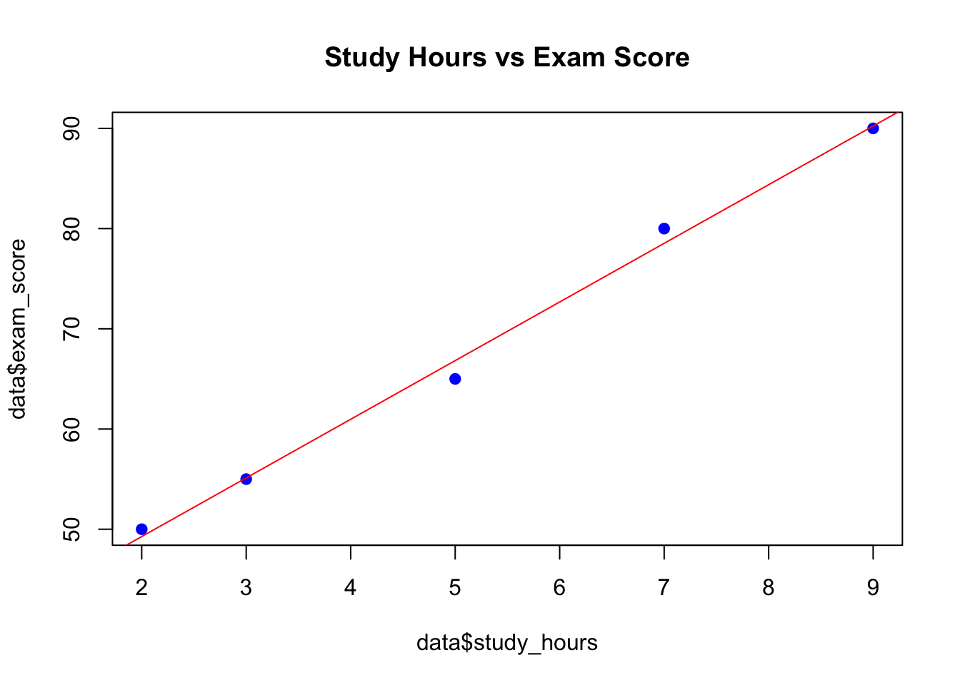
8.4.3 Example: Simple Linear Regression in R
A basic example of statistical modeling using linear regression to predict student exam scores based on study hours.
Code
# Sample dataset data<-data.frame( study_hours =c(2, 3, 5, 7, 9), exam_score =c(50, 55, 65, 80, 90))# Build a linear regression model model<-lm(exam_score~study_hours, data =data)# Summary of the model summary(model)
Call:
lm(formula = exam_score ~ study_hours, data = data)

Residuals:
      1       2       3       4       5
 0.7317 -0.1220 -1.8293  1.4634 -0.2439

Coefficients:
            Estimate Std. Error t value Pr(>|t|)
(Intercept)  37.5610     1.4429   26.03 0.000124 ***
study_hours   5.8537     0.2489   23.52 0.000169 ***
---
Signif. codes:  0 '***' 0.001 '**' 0.01 '*' 0.05 '.' 0.1 ' ' 1

Residual standard error: 1.426 on 3 degrees of freedom
Multiple R-squared:  0.9946,    Adjusted R-squared:  0.9928
F-statistic:   553 on 1 and 3 DF,  p-value: 0.0001685
Code
# Visualizing the relationship plot(data$study_hours, data$exam_score, col ="blue", pch =19, main ="Study Hours vs Exam Score")abline(model, col ="red")